Exercises - Chapter 8: Permutation Tests
Students:
- Henrique Aparecido Laureano
- Elainy Marciano Batista
- Heidi Mara do Rosário Souza
- Joubert Miranda Guedes
- Nicolas Romano
- Pedro Luciano de Oliveira Gomes
- Ricardo de Faria Souza
- Telma Tompson
- Thais Castelo Branco Monho
Exercises from chapter 8 of the book:
Maria L. Rizzo, 2008. Statistical Computing with R, Chapman & Hall/CRC, ISBN 1-58488-545-9, 393 pages.
Exercise 8.1
Implement the two-sample Cramér-von Mises test for equal distributions as a permutation test. Apply the test to the data in Examples 8.1 and 8.2.
Solution:
data("chickwts")

## Packages
library(latticeExtra)

## function: two-sample Cramér-von Mises test for equal distributions
cvm <- function(x, y, data){
  r <- 10000 # Permutation samples
  reps <- vector("numeric", r)
  n <- length(x)
  m <- length(y)
  v.n <- vector("numeric", n) # Replication vectors
  v1.n <- vector("numeric", n)
  v.m <- vector("numeric", m)
  v1.m <- vector("numeric", m)
  z <- c(x, y)
  N <- length(z)
  for (i in 1:n) v.n[i] <- ( x[i] - i )**2
  for (j in 1:m) v.m[j] <- ( y[j] - j )**2
  # Test statistic
  reps_0 <- ( (n * sum(v.n) + m * sum(v.m)) / (m * n * N) ) -
    (4 * m * n - 1) / (6 * N)
  for (k in 1:r) { # Permautation samples
    w <- sample(N, size = n, replace = FALSE)
    x1 <- sort( z[ w] )
    y1 <- sort( z[-w] )
    for (i in 1:n) { v1.n[i] <- ( x1[i] - i )**2 }
    for (j in 1:m) { v1.m[j] <- ( y1[j] - j )**2 }
    reps[k] <- ( (n * sum(v1.n) + m * sum(v1.m)) / (m * n * N) ) -
      (4 * m * n - 1) / (6 * N)
  }
  p <- mean( c(reps_0, reps) >= reps_0 )
  return(
    histogram(c(reps_0, reps) # Histogram
              , type = "density"
              , col = "#0080ff"
              , xlab = "Replicates of Cramér-Von Mises (CVM) statistic"
              , ylab = list(rot = 0)
              , main = paste0(
                "Data: ", data, "\n"
                , "Permutation distribution of CVM statistic")
              , sub = list(substitute(paste(hat(p), " = ",pvalue)
                                      , list(pvalue = p))
                           , col = 2)
              , panel = function(...){
                panel.histogram(...)
                panel.abline(v = reps_0, col = 2, lwd = 2)
              })
  )
}
## Data: Example 8.1
x <- with(chickwts, sort(as.vector(weight[feed == "soybean"])))
y <- with(chickwts, sort(as.vector(weight[feed == "linseed"])))

cvm_8.1 <- cvm(x, y, "Example 8.1")

## Data: Example 8.2
x <- with(chickwts, sort(as.vector(weight[feed == "sunflower"])))
y <- with(chickwts, sort(as.vector(weight[feed == "linseed"])))

cvm_8.2 <- cvm(x, y, "Example 8.2")

## Results
print(cvm_8.1, position = c(0, 0, .5, 1), more = TRUE)
print(cvm_8.2, position = c(.5, 0, 1, 1))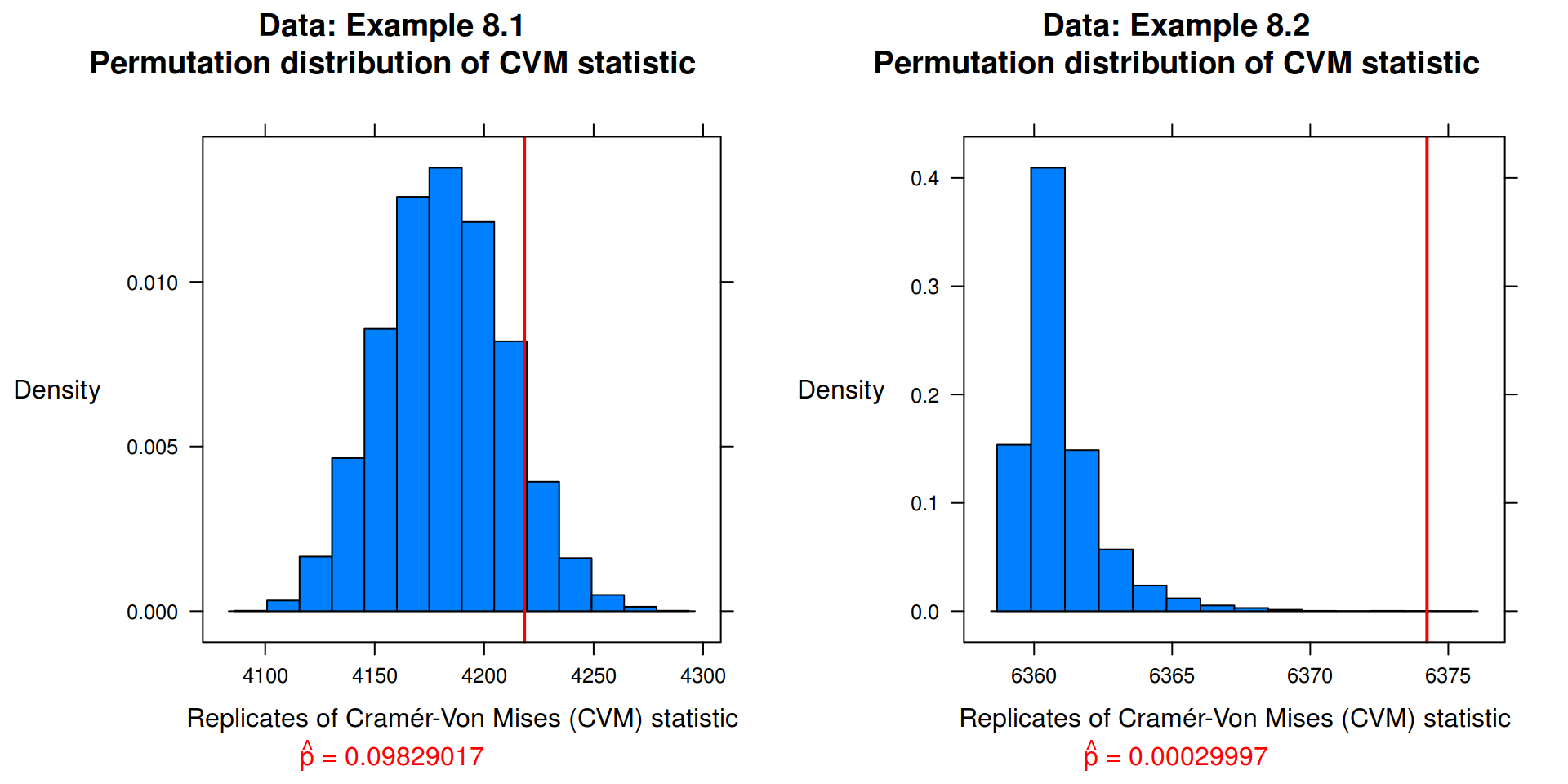
Exercise 8.2
Implement the bivariate Spearman rank correlation test for independence [255] as a permutation test. The Spearman rank correlation test statistic can be obtained from function cor with method = "spearman". Compare the achieved significance level of the permutation test with the p-value reported by cor.test on the same samples.
Solution:
data("iris")

## Dataset
z <- as.matrix(iris[1:50, 1:4])
x <- (z[ , 1:2])
y <- (z[ , 3:4])

cor(x,y, method = "spearman")
Petal.Length Petal.Width
Sepal.Length 0.2788849 0.2994989
Sepal.Width 0.1799110 0.2865359cor.test(x, y, method = "spearman", exact = FALSE)$estimate rho
0.8292811 ## Packages
library(boot)
## function: bivariate Spearman rank correlation test for independence
spear.cor <- function(z) {
rho.est <- function(z, i) { # Test statistic
x <- z[ , 1:2]
y <- z[i, 3:4]
return(cor.test(x, y, method = "spearman", exact = FALSE)$estimate)
}
perm <- boot(data = z # 10000 permutation samples
, statistic = rho.est
, sim = "permutation"
, R = 10000)
p <- with(perm, mean( c(t, t0) >= t0 )) # p-value
return(
histogram(with(perm, c(t, t0)) # Histogram
, type = "density"
, col = "#0080ff"
, xlab = "Replicates correlation"
, ylab = list(rot = 0)
, main = paste(
"Permutation distribution of the bivariate Spearman",
"rank correlation test")
, sub = list(substitute(paste(hat(p), " = ",pvalue)
, list(pvalue = p))
, col = 2)
, panel = function(...){
panel.histogram(...)
panel.abline(v = perm$t0, col = 2, lwd = 2)
})
)
}
spear.cor(z)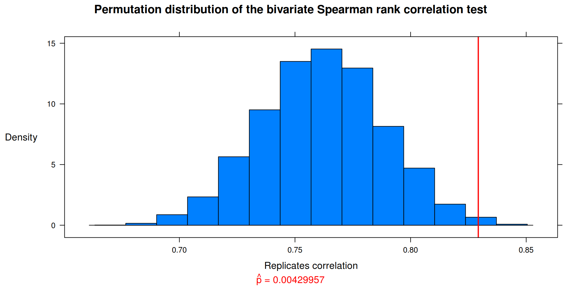
Exercise 8.3
The Count 5 test for equal variances in Section 6.4 is based on the maximum number of extreme points. Example 6.15 shows that the Count 5 criterion is not applicable for unequal sample sizes. Implement a permutation test for equal variance based on the maximum number of extreme points that applies when sample sizes are not necessarily equal.
Solution:
## Dataset
n_1 <- 20 # Defining the sample sizes
n_2 <- 30
x <- rnorm(n_1, 0, 5)
y <- rnorm(n_2, 0, 5)

## function: permutation test for equal variance based
##           on the maximum number of extreme points
count5 <- function(x, y) {
  count5test <- function(x, y) { # Test statistic
    X <- x - mean(x)
    Y <- y - mean(y)
    outx <- sum(X > max(Y)) + sum(X < min(Y))
    outy <- sum(Y > max(X)) + sum(Y < min(X))
    # Return 1 (reject) or 0 (do not reject H_{0})
    return( as.integer( max(c(outx, outy) ) > 5) )
  }
  r <- 10000 # Permutation samples
  z <- c(x, y)
  n <- length(z)
  reps <- vector("numeric", r)
  t0 <- count5test(x, y)
  for (i in 1:r){ # Permutation test
    k = sample(n, size = length(x), replace = FALSE)
    reps[i] = count5test(z[k], z[-k])
  }
  p <-
    ifelse(t0 == 0, mean( c(t0, reps) > t0 ), mean( c(t0, reps) >= t0 ))
  return(
    histogram(c(t0, reps) # Histogram
              , type = "density"
              , col = "#0080ff"
              , xlab = "Replicates of the Count 5 test"
              , ylab = list(rot = 0)
              , main = "Permutation distribution of the Count 5 test"
              , sub = list(substitute(paste(hat(p), " = ",pvalue)
                                      , list(pvalue = p))
                           , col = 2)
              , panel = function(...){
                panel.histogram(...)
                panel.abline(v = t0, col = 2, lwd = 2)
              })
  )
}
count5(x, y)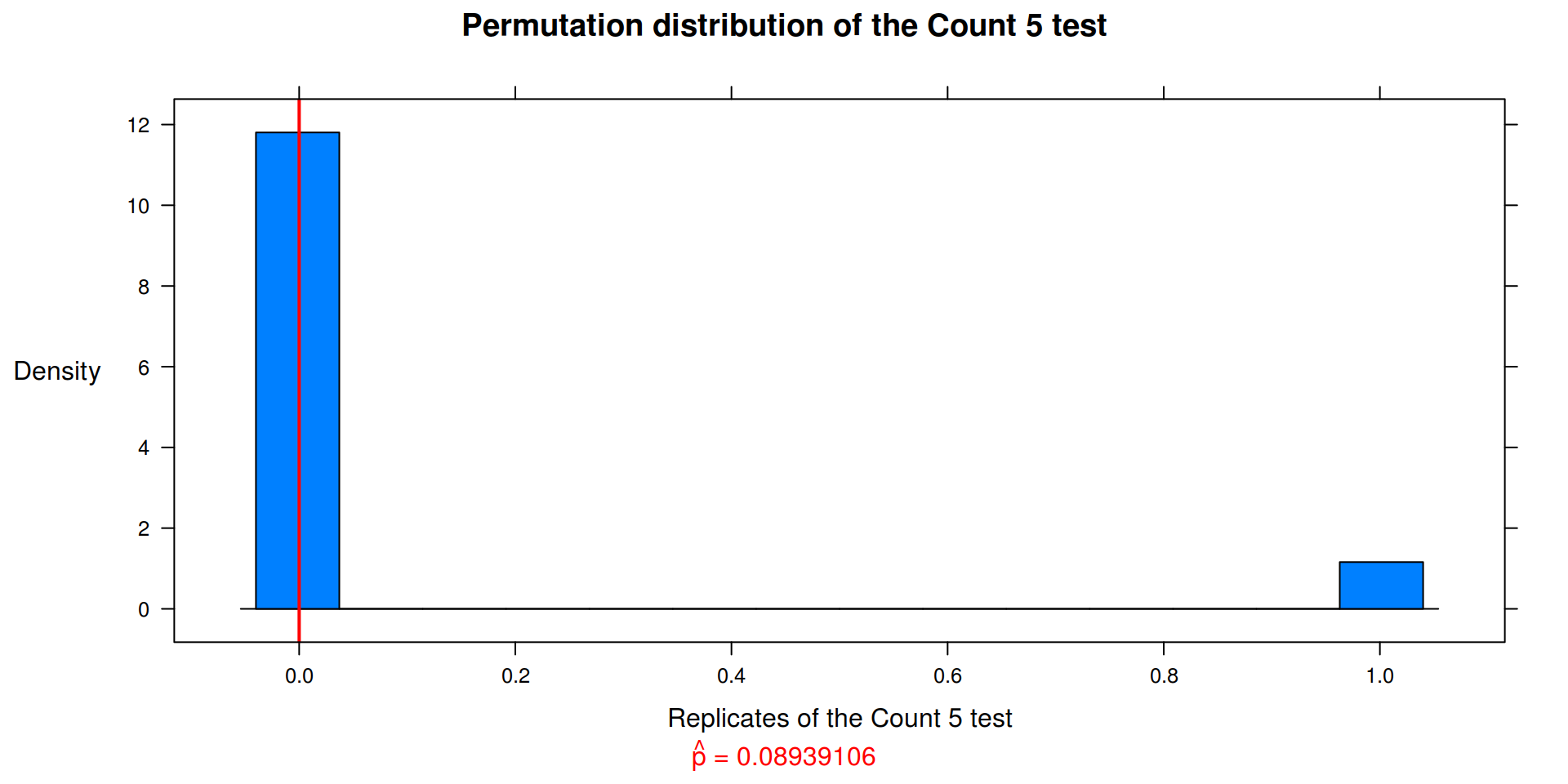
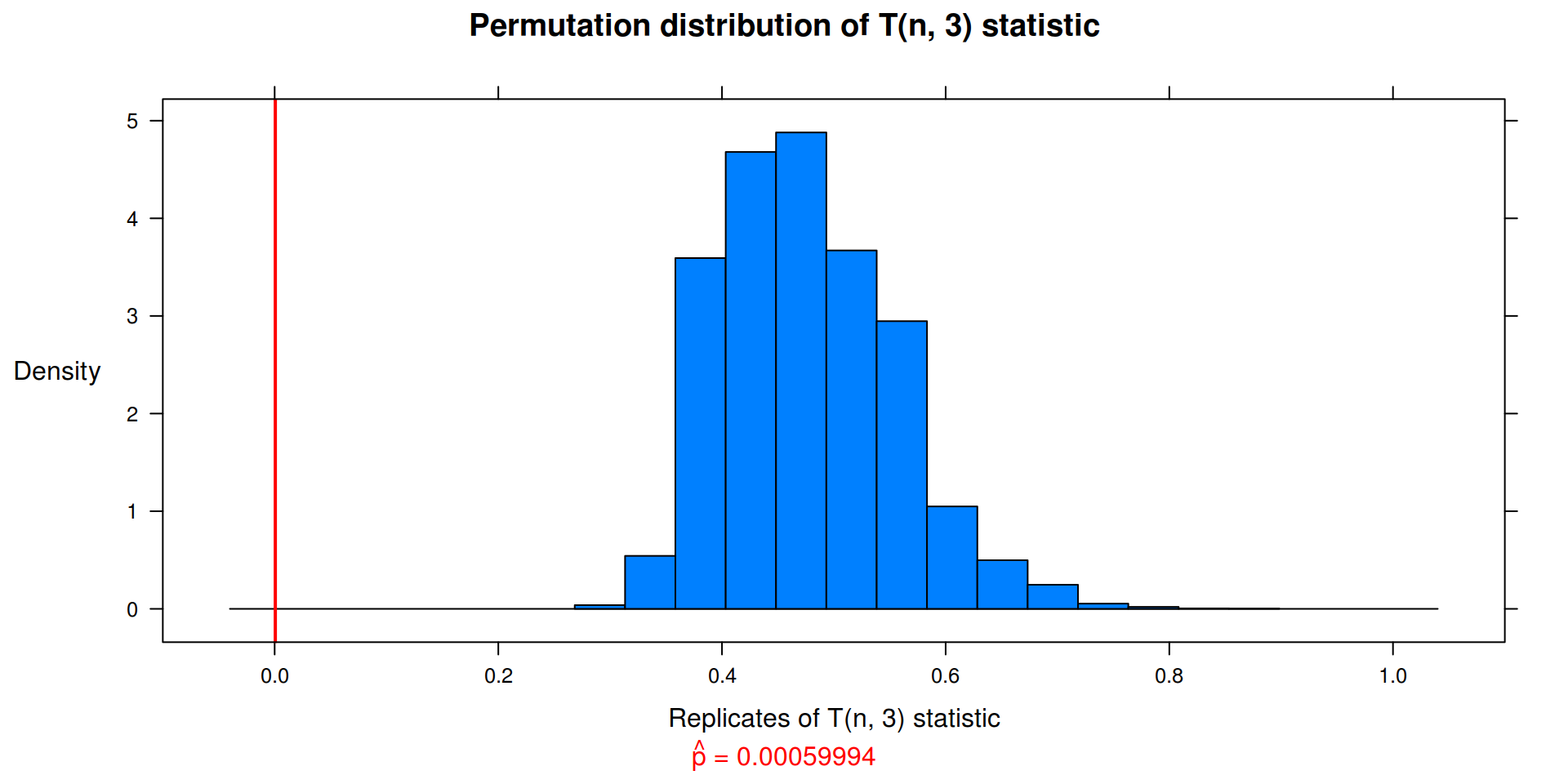
Exercise 8.4
Complete the steps to implement a \(r^{th}\) -nearest neighbors test for equal distributions. Write a function to compute the test statistic. The function should take the data matrix as its first argument, and an index vector as the second argument. The number of nearest neighbors r should follow the index argument.
Solution:
data("chickwts")

## Dataset
x <- with(chickwts, as.vector(weight[feed == "sunflower"]))
y <- with(chickwts, as.vector(weight[feed == "linseed"]))
z <- cbind( c(x, y), rep(0, length(c(x, y))) )

## Packages
library(boot)
library(FNN)
library(latticeExtra)

## function: r^{th} -nearest neighbors test for equal distributions
my.knn <- function(z, nn) {
  t_n.i <- function(z, nn, i) {
    n_g <- nrow(z) / 2 # length x and length y
    n <- nrow(z)
    z <- z[i, ]
    z <- cbind(z, rep(0, n))
    knn <- get.knn(z, k = nn) # Obtaining the k nearest neighbors
    n_1 <- knn$nn.index[1:n_g, ]       # Dividing x
    n_2 <- knn$nn.index[(n_g + 1):n, ] # and y
    i_1 <- sum(n_1 < n_g + .5) # Obtaining the sum of
    i_2 <- sum(n_2 > n_g + .5) # the indicator functions
    return( (i_1 + i_2) / (nn * n) ) # Test statistic
  }
  perm <- boot(data = z # 10000 permutation samples
               , statistic = t_n.i
               , sim = "permutation"
               , R = 10000
               , nn = 3)
  p <- with(perm, mean( c(t, t0) >= t0 )) # p-value
  return(
    histogram(with(perm, c(t, t0)) # Histogram
              , type = "density"
              , col = "#0080ff"
              , xlim = c(-.1, 1.1)
              , xlab = paste0("Replicates of T(n, ", nn, ") statistic")
              , ylab = list(rot = 0)
              , main = paste0("Permutation distribution of T(n, "
                              , nn, ") statistic")
              , sub = list(substitute(paste(hat(p), " = ", pvalue)
                                      , list(pvalue = p))
                           , col = 2)
              , panel = function(...){
                panel.histogram(...)
                panel.abline(v = p, col = 2, lwd = 2)
              })
  )
}
my.knn(z, 3) # k (or r) nearest neighbors = 3