Bootstrap
Resampling methods treat samples as a finite population, from which samples are taken to estimate features and make inferences about this population.
To generate a random bootstrap sample by \(x\) resampling, generate \(n\) uniformly distributed random integers in the set \(1, ..., n{}\) and select the bootstrap sample as \(x^{*} = (x_{i_{1}}, ..., x_{i_{n}})\).
\[ F \rightarrow X \rightarrow F_{n} \\ F_{n} \rightarrow X^{*} \rightarrow F_{n}^{*}. \]
Example 1 Suppose we observe the following data:
\(x = {2, 2, 1, 1, 5, 4, 4, 3, 1, 2}\).
Resampling from \(x\), we select \(\{1, 2, 3, 4, 5\}\) with probabilities \(\{0.3, 0.3, 0.1, 0.2, 0.1\}\). The \(F_{X^{*}}(x)\) distribution of a sample taken at random is exactly the function \(F_{n}\):
\[ F_{X^{*}}(x) = F_{n}(x) = \begin{cases} 0.0 & x < 1; \\ 0.3 & 1 \leq x < 2; \\ 0.6 & 2 \leq x < 3; \\ 0.7 & 3 \leq x < 4; \\ 0.9 & 4 \leq x < 5; \\ 1.0 & x \geq 5. \end{cases} \]Bootstrap estimation of standard error
The bootstrap estimate of the standard error of an estimator \(\hat{\theta}\) is the sample standard error of the bootstrap replicates \(\hat{\theta}^{(1)}, ..., \hat{\theta}^{(B)}\):
\[ \text{se}(\hat{\theta}^{*}) = \sqrt{\frac{1}{B - 1} \sum_{b = 1}^{B} (\hat{\theta}^{(b)} - \bar{\theta}^{*})^{2}}, \\ \bar{\theta}^{*} = \frac{1}{B} \sum_{b = 1}^{B} \hat{\theta}^{(b)}. \]
Where \(B\) is the number of replicates.
Example 2 (Correlation)
lattice::xyplot(dist ~ speed, cars, pch = 16, ylab = list(rot = 0))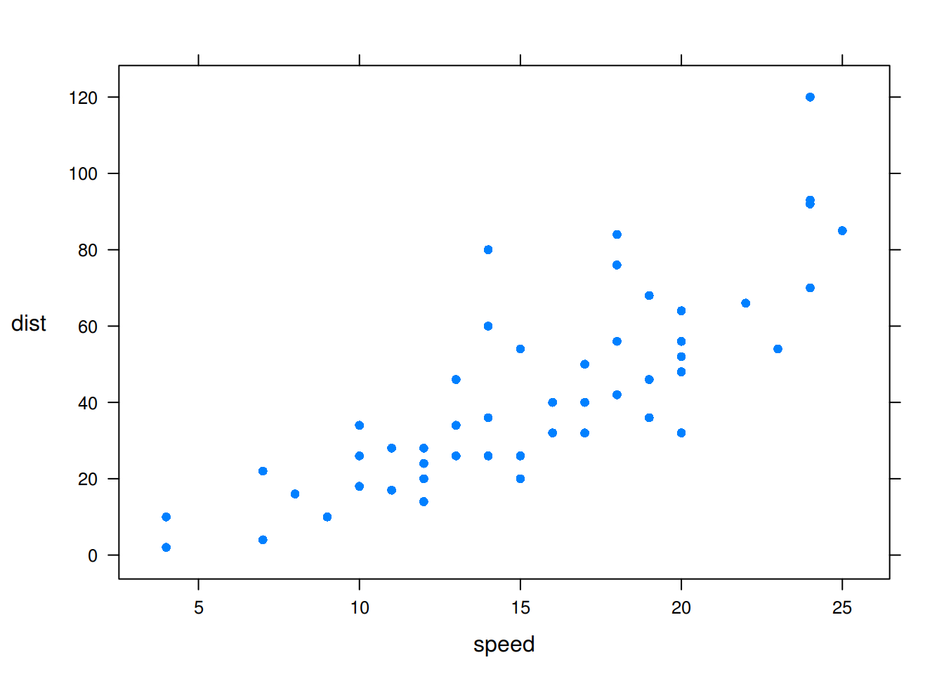
Figure 1: A scatterplot of the speed and dist variables of the cars dataframe.
set.seed(1)
B <- 10e3
boot.corr <- vector('numeric', B)
for (b in 1:B){
  ind <- sample(nrow(cars), replace = TRUE)
  boot.corr[b] <- with(cars[ind, ], cor(dist, speed))
}
(theta.star <- mean(boot.corr))
[1] 0.8062458(se.theta.star <- sd(boot.corr))[1] 0.04782856Bootstrap estimation of bias
The definition of bias is given by:
\[ B(\hat{\theta}) = E(\hat{\theta}) - \theta. \]
Thus, the bootsrap estimate of bias is:
\[ \hat{B(\hat{\theta})} = \bar{\hat{\theta}^{*}} - \theta, \]
expression in which \(\bar{\hat{\theta}^{*}} = \frac{1}{B} \sum_{b = 1}^{B} \hat{\theta}^{(b)}\) and \(\hat{\theta}\) is the estimate calculated using the original sample.
Every statistic is an unbiased estimator of its expected value, and in particular, the sample mean of a random sample is an unbiased estimator of the mean of the distribution. An example of a biased estimator is the maximum likelihood estimator of variance, \(\hat{\sigma}^{2} = \frac{1}{n} \sum_{i = 1}^{n} (X_{i} - \bar{X})^{2}\), which has expected value \((1 - 1/n) \sigma^{2}\). Thus, \(\hat{\sigma}^{2}\) underestimates \(\sigma^{2}\), and the bias is \(-\sigma^{2}/n\).
In bootstrap \(F_{n}\) is sampled in place of \(F_{X}\), so we replace \(\theta\) with \(\hat{\theta}\) to estimate the bias. Positive bias indicates that \(\hat{\theta}\) on average tends to overestimate \(\theta\).
Example 3 (Correlation)
theta.star - with(cars, cor(dist, speed))[1] -0.0006490941